| Updating Python Code 6.1 (p.190) for Figure 6.7 (p.88) |
|
<コード code6.1.py>
磁気コンパス濃度の自差グラフをフーリェ級数でフィッティング(あてはめ)をします。
Berendsen氏のコードを下に記します。
- from scipy import optimize
- # data from compass corrections:
- x = arange(0., 365., 15.)
- y = array([-1.5,-0.5,0.,0.,0.,-0.5,-1.,-2.,
-3.,-2.5,-2.,-1.,
0.,0.5,1.5,2.5,2.0,2.5,
1.5,0.,-0.5,-2.,-2.5,-2.,-1.5])
- def fitfun(x,p):
- phi = x*pi/180.
- result = p[0]
- for i in range(1,5,1):
- result = result+[2*i-1]*np.sin(i*phi)+p[2*i]*np.cos(i*phi)
- return result
- def residual(p): return y-fitfun(x, p)
- pin = [0.]*9 # initial guess
- output = optimize.leastsq(residual, pin)
- print(output)
- pout = output[0] # optimized params
- def fun(x): return fitfun(x, pout) # for plotting
このコードなら無事通るはずと思っていましたが、実際には import numpy as np を加え、np.arange, np.array, np.pi
に直して正常終了しました。
テキストでは省略してあったグラフィックス部分については、
import matplotlib.pyplot as plt を先頭に書き加え、次のコードを追加して右図を得ることができました。
|
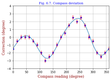
<グラフィックス出力>
4次の高調波まで取り入れたデータ・フィッティングです。
|
|
<グラフィックス部のコード>
- t = np.arange(0.,361.,1.)
- plt.xlim(0,360)
- plt.ylim(-4,4)
- plt.plot(t, fun(t))
- for i in range(25):
- plt.plot(x[i],y[i],marker="o",markersize=5,color="blue")
- xs = np.array([x[i], x[i]])
- ys = np.array([y[i]-0.25, y[i]+0.25])
- plt.plot(xs,ys,color="red")
- font1 = {'family':'serif','color':'blue','size':11}
- font2 = {'family':'serif','color':'darkred','size':12}
- plt.title("Fig. 6.7. Compass deviation", fontdict = font1)
- plt.xlabel("Compass reading (degree)", fontdict = font2)
- plt.ylabel("Correction (degree)", fontdict = font2)
- plt.grid()
- plt.show()
|
<コメント1>
- お恥ずかしい話ですが y のデータを一つ書き落としたためにエラーが出ました。
operands could not be broadcast together with shapes (24,) (25,) というメッセージからすみやかに気づくべきでした。
- 非線形問題には optimize.least_squares を使うとのことです。
|
|
<コメント2>
optimize.curve_fit でも解けました。主な変更箇所を下に記します。
- def fitfun(x,p0,p1,p2,p3,p4,p5,p6,p7,p8):
- phi = x*np.pi/180.
- s = p0 + p1*np.sin(phi) + p2*np.cos(phi) + p3*np.sin(2*phi) + p4*np.cos(2*phi)
- s += p5*np.sin(3*phi) + p6*np.cos(3*phi) + p7*np.sin(4*phi) + p8*np.cos(4*phi)
- return s
- output = optimize.curve_fit(fitfun, x, y)
- pout = output[0]
- def fun(x): return fitfun(x, *pout)
|
<コメント3>
fitfunを次のように定義するとスマートにいきます(nfree=9)。
ただし初期値 pini も渡しておかないと Unable to determine number of fit parameters というメッセージが出ます。
- def fitfun(x, *q):
- phi = x*np.pi/180.
- i = 0
- j = 0
- s = q[0]
- while True:
- if i>=nfree-1:
- break
- i += 1
- w = q[i]
- j = (i+1) // 2
- if i%2 != 0:
- s += w*np.sin(j*phi)
- else:
- s += w*np.cos(j*phi)
- return s
- pini = [0.]*nfree
- output = optimize.curve_fit(fitfun, x, y, pini)
|