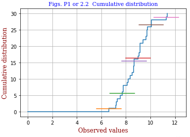
30 data points x_i (i=1..N) are arranged in increasing order and x is plotted against i. The author made a simulation using random numbers.

1. from scipy import *
2. x = 8.5 + randn(30)
3. xr = x.sort().round(2)
4. from plotsvg import *
5. autoplotc(xr,title='Cumulative distribution')

1. code 2.1bb.py: Berendsen's data are written to a csv file (contents) and then fed to the program. The result is shown in the right.
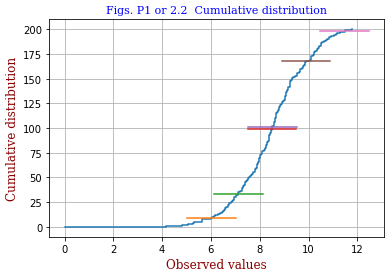
2. code 2.1cc.py: A set of random data is arranged, The x-axis is drawn in two ways. One is an ordinary axis with homogeneous spacings. The x-axis of the other is inhomogeneous such that spacings are narrower near 0% and 100% and wide at 50%, the details are explained elsewhere. The results are shown by two graphs in the right.

The tasks used for producing the graphs have been divided into the following modules. The modules are to be imported if necessary.

• hwbfiles...Read a textfile
• hwblines...Convert the original data (x_i,y_i) to plot data (u_k,v_k). Here v_k is different from v_m if m<>k. The spacing of the v-axis may be unity or may be inhomogeneous decreasing toward 0% and 100%.
• statpos...indicating the positions for the mean, median, mode, and standard deviation.

Let the frequency y_i be coverted to the probability P_i=(i-1/2)/n  (i=1,..,n) and plotted against i. (Please check Wikipedia, Normal probability plot.) The procedure may be made simple if the data are plotted on the so-called probability paper. If the data obey the normal distribution, the points tend to align in a straight line.
The procedure may be even simpler if the computer is used: The data are converted in accordance with the following equation.

The code code2.2cc.py has given the result as shown right.