|
<code7.3.py>
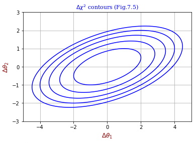
For two fitting parameters the chi squared is given by
Δχ2=ΣijBijθiθj
Figure 7.5 is the result for B=[[1,-1],[-1,4]].
In his code7.3.py Dr. Berendsen uses his original 'contour' for obtaining points on the contour.
He says that 'autoplotp' will do the plotting task but it cannot be located.
With the popular PyPlotLib I could get the picture in the right.
A primary change to his code7.3.py is that 'xlist, ylist' are returned instead of the single 'data'.
The plotting program is shown below.
- def contour:
- ......(Original code 7.3 with modifications)
- def fxy(x,y):
- v = np.array([[x,y]])
- w = np.dot(v, matrx @ v.T)
- return w
- plt.xlim(-5., 5.)
- plt.ylim(-3., 3.)
- xycenter= np.array([0.0, 0.0])
- for i in range(1,6):
- z = i
- xlist,ylist = contour(fxy,z,xycenter)
- plt.plot(xlist,ylist,color='blue')
- font1 = {'family':'serif','color':'blue','size':11}
- font2 = {'family':'serif','color':'darkred','size':12}
- plt.title(r"$\Delta \chi^2$ contours (Fig.7.5)", fontdict = font1)
- plt.xlabel(r"$\Delta \theta_1$", fontdict = font2)
- plt.ylabel(r"$\Delta \theta_2$", fontdict = font2)
- plt.grid()
- plt.show()
|
<Graphics output>
<Remark>
For fxy(x,y)=v B vT, v is a row vector, [x,y], and vTis a column vector.
If the matrix B is specified, it is possible to expand fxy to obtain
fxy=x2-2xy+4y2
but matrix computation is adopted in the left for the purpose of excercise.
The modifications to the original code 7.3 are as folows
- 'import numpy as np' is added
- 'import matplotlib.pyplot as plt' is added
- 'return data' is replaced by 'return xlist,ylist'
|
|
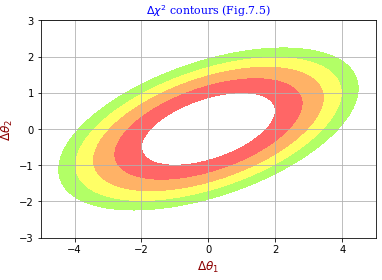
<Another method using matplotlib.contourf>
Plotting is included. v B vT is calculated for the vector v.
- import numpy as np
- import matplotlib.pyplot as plt
- matrx = np.array([[1.0, -1.0],[-1.0, 4.0]])/3.0
- nxpt = 201; nypt = 121
- x = np.linspace(-5., 5.,nxpt)
- y = np.linspace(-3., 3.,nypt)
- z = np.zeros((nypt,nxpt))
- xx, yy = np.meshgrid(x,y)
- def findz(x,y):
- for i in range(nypt):
- yi = y[i,0]
- for j in range(nxpt):
- xj = x[0,j]
- v = np.array([xj,yi])
- w = matrx @ v.T
- z[i,j] = np.dot(v, w)
- return z
- zz = findz(xx, yy)
- # zz = (xx**2 - 2.*xx*yy + 4.*yy**2)/3.0
- xycenter= np.array([0.0, 0.0])
- figure = plt.contourf(xx,yy,zz,levels=[1.,2.,3.,4.,5.],\
- colors=['#FF6666','#FFB266','#FFFF66','#B2FF66', \
- '#66FF66','#66FFFF'])
- font1 = {'family':'serif','color':'blue','size':11}
- font2 = {'family':'serif','color':'darkred','size':12}
- plt.title(r"$\Delta \chi^2$ contours (Fig.7.5)", fontdict = font1)
- plt.xlabel(r"$\Delta \theta_1$", fontdict = font2)
- plt.ylabel(r"$\Delta \theta_2$", fontdict = font2)
- plt.grid()
- plt.show()
|
<Graphics output>
<Remark>
Moving # of line 19 to line 18 changes the matrix calculation to polynomial calculation.
|