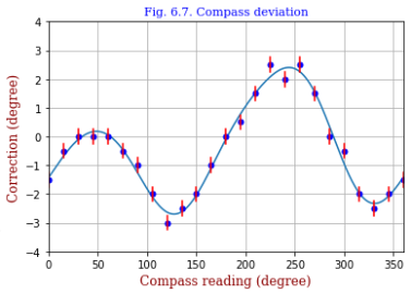
The deviation of magnetic compass is fitted by a Fourier series, for which Dr. Berendsen wrote the following code.

1. from scipy import optimize
2. # data from compass corrections:
3. x = arange(0., 365., 15.)
4. y = array([-1.5,-0.5,0.,0.,0.,-0.5,-1.,-2., -3.,-2.5,-2.,-1.,
   0.,0.5,1.5,2.5,2.0,2.5, 1.5,0.,-0.5,-2.,-2.5,-2.,-1.5])
5. def fitfun(x,p):
6.    phi = x*pi/180.
7.    result = p[0]
8.    for i in range(1,5,1):
9.      result = result+[2*i-1]*np.sin(i*phi)+p[2*i]*np.cos(i*phi)
10.    return result
11. def residual(p): return y-fitfun(x, p)
12. pin = [0.]*9    # initial guess
13. output = optimize.leastsq(residual, pin)
14. print(output)
15. pout = output[0]    # optimized params
16. def fun(x): return fitfun(x, pout)   # for plotting

For the graphics part left out in the book, I added the following line
     import matplotlib.pyplot as plt
and the lines to obtain the graph in the right.

Data fit including harmonics up to fouth order.

1. t = np.arange(0.,361.,1.)
2. plt.xlim(0,360)
3. plt.ylim(-4,4)
4. plt.plot(t, fun(t))
5. for i in range(25):
6.    plt.plot(x[i],y[i],marker="o",markersize=5,color="blue")
7.    xs = np.array([x[i], x[i]])
8.    ys = np.array([y[i]-0.25, y[i]+0.25])
9.    plt.plot(xs,ys,color="red")
10. font1 = {'family':'serif','color':'blue','size':11}
11. font2 = {'family':'serif','color':'darkred','size':12}
12. plt.title("Fig. 6.7. Compass deviation", fontdict = font1)
13. plt.xlabel("Compass reading (degree)", fontdict = font2)
14. plt.ylabel("Correction (degree)", fontdict = font2)
15. plt.grid()
16. plt.show()

• I failed to include one of y data and came up with the message
    operands could not be broadcast together with shapes (24,) (25,)
  The error should have been fixed more quickly.

• 'optimize.least_squares' should be used for nonlinear problems.

The problem could be solved also with optimize.curve_fit with the following changes.

1. def fitfun(x,p0,p1,p2,p3,p4,p5,p6,p7,p8):
2.    phi = x*np.pi/180.
3.    s = p0 + p1*np.sin(phi) + p2*np.cos(phi) + p3*np.sin(2*phi) + p4*np.cos(2*phi)
4.    s += p5*np.sin(3*phi) + p6*np.cos(3*phi) + p7*np.sin(4*phi) + p8*np.cos(4*phi)
5.    return s
6. output = optimize.curve_fit(fitfun, x, y)
7. pout = output[0]
8. def fun(x): return fitfun(x, *pout)

It is a nice idea to define fitfun in the following way (nfree=9). Do not forget to define the initial value, pini. Otherwise you may encounter with the message
     'Unable to determine number of fit parameters'

1. def fitfun(x, *q):
2.    phi = x*np.pi/180.
3.    i = 0
4.    j = 0
5.    s = q[0]
6.    while True:
7.       if i>=nfree-1:
8.          break
9.       i += 1
10.       w = q[i]
11.       j = (i+1) // 2
12.       if i%2 != 0:
13.          s += w*np.sin(j*phi)
14.       else:
15.          s += w*np.cos(j*phi)
16.    return s
17. pini = [0.]*nfree
18. output = optimize.curve_fit(fitfun, x, y, pini)